Polynomial Regression
Example: QUADRATIC MODEL FOR
PREDICTING THE US POPULATION
> setwd("C:\Users\baron\624 Data Analysis\data")
> read.csv("USpop.csv")
Year Population
1 1790 3.9
2 1800 5.3
3 1810 7.2
4 1820 9.6
5 1830 12.9
6 1840 17.1
7 1850 23.2
8 1860 31.4
9 1870 38.6
10 1880 50.2
11 1890 63.0
12 1900 76.2
13 1910 92.2
14 1920 106.0
15 1930 123.2
16 1940 132.2
17 1950 151.3
18 1960 179.3
19 1970 203.3
20 1980 226.5
21 1990 248.7
22 2000 281.4
23 2010 308.7
> Data = read.csv("USpop.csv")
> names(Data)
[1] "Year"
"Population"
> attach(Data)
> plot(Year,Population)
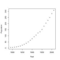
> # LINEAR MODEL
> lin = lm(Population ~ Year)
> summary(lin)
Call:
lm(formula = Population ~ Year)
Residuals:
Min 1Q
Median 3Q Max
-27.774 -24.872
-6.295 18.374 55.087
Coefficients:
Estimate
Std. Error t value
(Intercept) -2.481e+03
1.672e+02 -14.84
Year
1.360e+00 8.794e-02 15.47
Pr(>|t|)
(Intercept) 1.33e-12 ***
Year 5.93e-13 ***
---
Signif. codes:
0 ‘***’ 0.001 ‘**’ 0.01
‘*’ 0.05 ‘.’
0.1 ‘ ’ 1
Residual standard error: 27.97 on 21 degrees of freedom
Multiple R-squared:
0.9193, Adjusted
R-squared: 0.9155
F-statistic: 239.3 on 1 and 21 DF, p-value: 5.927e-13
> abline(lin,col="red",lwd=3)
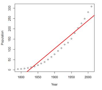
Ø #
Clearly, the linear model is too inflexible and restrictive, it does not
provide a good fit. This is underfitting. Notice, however, that R2
in this regression is 0.9193. Without looking at the plot, we could have
assumed that the model is very good!
> predict(lin,data.frame(Year=2020))
1
267.2166
Ø # This
is obviously a poor prediction. The US population was already 308 million
during the most recent Census.
Ø So,
we probably omitted an important predictor. Residual plots will help us
determine which one.
Ø Let’s
produce various related plots.
Ø Partition
the graphics window into 4 parts and use “plot”.
> par(mfrow=c(2,2))
> plot(lin)
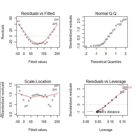
Ø # The
first plot shows that a quadratic term has been omitted although it is
important in the population growth.
Ø # So,
fit a quadratic model.
Ø Command
I(…) means “inhibit interpretation”, it forces R to understand (…) literally,
as Year squared.
> quadr = lm(Population ~ Year + I(Year^2))
> par(mfrow=c(1,1))
> plot(Year,Population)
Ø # Now
let’s plot the fitted curve. Obtain fitted values.
> Yhat = fitted.values(quadr)
> Yhat
1 2
3 4
6.490870 5.870040
6.603913 8.692490
5 6 7 8
12.135771 16.933755
23.086443 30.593834
9 10 11 12
39.455929 49.672727
61.244229 74.170435
13 14 15 16
88.451344 104.086957
121.077273 139.422292
17 18 19 20
159.122016 180.176443 202.585573 226.349407
21 22 23
251.467945 277.941186 305.769130
> lines(Year,Yhat,col="blue",lwd=3)
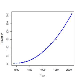
# This looks like a very good
fit! Only during WWII, the population grew at a rate slightly below the
quadratic trend, although it quickly caught up with it during the Baby Boom.
> summary(quadr)
Call:
lm(formula = Population ~ Year + I(Year^2))
Residuals:
Min 1Q
Median 3Q Max
-7.8220 -0.7130
0.5961 1.8344 3.7487
Coefficients:
Estimate
Std. Error t value
(Intercept)
2.194e+04 5.795e+02 37.87
Year
-2.438e+01 6.105e-01 -39.94
I(Year^2)
6.774e-03 1.606e-04 42.17
Pr(>|t|)
(Intercept) <2e-16
***
Year <2e-16
***
I(Year^2) <2e-16
***
---
Signif. codes:
0 ‘***’ 0.001 ‘**’ 0.01
‘*’ 0.05 ‘.’
0.1 ‘ ’ 1
Residual standard error: 3.023 on 20 degrees of freedom
Multiple R-squared:
0.9991, Adjusted
R-squared: 0.999
F-statistic: 1.113e+04 on 2 and 20 DF, p-value: < 2.2e-16
Ø A
higher R-squared is not surprising. It will always increase when we add new
variables to the model. The fair criterion is Adjusted R-squared, when we
compare models with a different number of parameters. Quadratic model has
Adjusted R-squared = 0.999 comparing with 0.9155 for the linear model.
> predict(quadr,data.frame(Year=2020))
1
334.9518
Ø Now,
this is a reasonable prediction for the year 2020.
>
predict(quadr,data.frame(Year=2020),interval="confidence")
fit lwr
upr
1 334.9518 330.6373 339.2663
>
predict(quadr,data.frame(Year=2020),interval="prediction")
fit lwr
upr
1 334.9518 327.311 342.5925
Ø Are
the confidence and predictions intervals valid here? We’ll discuss regression
assumptions next time.